
This post was written for the Q# Advent Calendar 2018. Check out the calendar for other posts.
Measurements of a quantum system are weird. It is mind-boggling that our classical world is somehow a manifestation of the counter-intuitive rules of quantum mechanics. When the classical world attempts to measure what’s in a quantum world, we obtain classical information and inevitably disturb the original system. (And we engineers are trying to build a computer out of this phenomenon!)
There have been many interpretations of measurements. Interference as an explanation was one of the topics that came up in discussions among our colleagues. As a “classically-trained” physicist (pun-intended), namely trained on approaches using wavefunctions, the Schrödinger equation, operators, the Copenhagen interpretation, etc., interference was an unfamiliar concept. I started learning from Scott Aaronson’s lectures about a new approach to teaching quantum mechanics that emphasizes the difference between classical probabilities and quantum probabilities. As I’ll explain later, this difference is what gives rise to interference effects in quantum mechanics. We’ll fast forward some fundamentals and talk about measurements and interference.
Learning together
The below writing is part of the tutorial for the Quantum Computing Study Group organized by The Garage at Microsoft. This is a community of learners meeting together to study different aspects of quantum computing, spanning software, hardware, mathematics and physics (see syllabus below). I’ve had the pleasure to lead sessions in Silicon Valley and the writing of the tutorial. We are collaborating across the globe with our colleagues in the India Garage. From these study groups, our employees began with no background in quantum computing, and worked to the point of being able to teach and write programs in Q#. The Garage also runs Microsoft’s annual hackathon. There were some quantum projects from this year’s hackathon. I want to give a shout out to a few colleagues from our Silicon Valley study group, Mario Inchiosa, Difu Su, Johnathan Tan and Hans Wang, who contributed to the Superdense Coding in the Quantum Katas, which are public programming exercises for learning Q# and quantum computing.
Two discoveries I made during my study: 1. Even if you are a physicist professionally, you may not know how quantum computers work. 2. You don’t have to have a degree in physics to study and understand quantum computing. This is an intellectually interesting subject made into something practical. I would recommend anyone to learn it.

TL;DR
Sections 1 and 2 explain the conventional construction of quantum mechanics and background on measurement. Feel free to skip these to look at the more interesting (or more unfamiliar) sections 3 and 4 on probability theory and interference. Section 5 shows where to find Q# exercises on measurement.
1. Some background
Typically, physicists learn the subject in a chronological order – how the field of Physics has developed through time. Because physicists were used to classical phenomena, experimental results of quantum mechanical phenomena appeared to be surprising when they were first discovered (look up the “UV Catastrophe”, “photoelectric effect”, “Compton Effect” and “interference of light at low intensity”). Physicists in the early 1900s naturally attempted to explain the results using classical methods.
One of the historical approaches to describe quantum phenomena is using wavefunctions. Physicists in the early 1900s found that quantum particles behave like waves. This means a quantum system can be described using a wave equation – the Schrödinger equation. Here is the Schrödinger equation for a non-relativistic particle in an external potential:

where 


The Schrödinger equation has a very interesting property called “linearity”. If we find two solutions 


The superposition behavior is written as
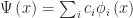
where we’re working in 1D (hence, x instead of r) for simplicity. Here, 


In terms of a qubit, the above equation is reflected by superposition of states, such as in 
To obtain the value of the coefficient of each possible basis state, one needs to find how much overlap there is between each basis state 


In Dirac notation, 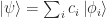

2. Measurement – not a gate
Measurements are different from gates. Gates are unitary which makes operations reversible. Gates acting upon a quantum system do not destroy the system or make connections between the system and the outside world. Applying a gate does not lose information. By contrast, when we in the outside world want to obtain information from the system, we need to measure it. However, measuring a system brings it into contact with the outside world, irrevocably destroying information. Thus, measurement is, in general, not reversible – the system cannot be brought back to its state before the measurement. One consequence of this difference is that a measurement cannot be operated with a gate. It is an interaction between the system and its environment. A parameter or physical variable measured from a quantum system is called an “observable” (because we can observe it). Momentum, mass, velocity and energy are all observables.
If we use the wavefunction approach, we can derive the value we’d expect to measure for a large number of measurements of a given observable, M. The expectation value can be obtained as
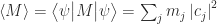
where 


In our two-qubit system, a state is described by a superposition of four basis states, i.e.

with coefficients 

After such a measurement, there are only two possible states that can exist in the system. The state becomes
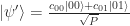
The denominator is there to keep the probability normalized. A measurement collapses a state 
Math insert – Hermitian operator
Recall that a gate is a unitary matrix, U, such that 

An observable corresponds to a Hermitian matrix, M, such that 

This number, m, is the value of the observable M that one would measure if the system were in state
The operator corresponding to an observable is required to be Hermitian, because measurement results or observables need to be real numbers. Here’s the proof that the measurement operator must be Hermitian:

If 


This must hold for any state
3. The 2-norm approach – an alternative way to teach and learn quantum mechanics
Now that we are in the 21st century, quantum phenomena are no longer so strange to physicists. With all the knowledge we have accumulated from the past, perhaps there is a more straightforward way to learn quantum mechanics, without the need to think about wavefunctions right away.
Essentially, we can start by generalizing probability theory. In our experience, probabilities are always positive and sum to 1. This is called the “1-norm” condition:

In quantum mechanics, we don’t work directly with probabilities. Instead, we work with “amplitudes”. The square of an amplitude is a probability, so we require that squares of the amplitudes sum to 1. This is called the “2-norm” condition (where “2” refers to the fact that we’re squaring the amplitudes):

One thing to note here is that when we talk about “squaring” a number, we actually mean taking the “modulus squared” (or the “square of the magnitude”) , which is done by multiplying it by its complex conjugate: 
Because of the 2-norm condition, an amplitude can be a positive, negative or even complex number. In the example above, we wrote the amplitudes as 
The complex number 


This alternative quantum mechanics introduction bypasses wavefunction derivations. It puts up front that the universe behaves according to the 2-norm condition with a set of axioms. This allows us to see some fundamental quantum mechanical behaviors without dealing with more complicated systems, such as particles in an external potential.
4. Interference
The key of a generalized probability theory is that probability is equal to the square of magnitude of amplitude, so the square of amplitude must be a positive number between 0 and 1. Here, we’re going to look at the idea of interference between different possibilities, which is something that is typical of quantum mechanics, but not of classical probability theory. Interference occurs because we use amplitudes, rather than probabilities, and amplitudes can be negative or complex. Let’s use a metaphorical example to illustrate this abstract idea.
Say Bob is someone who may like sports and/or computer games. He has a 70% chance of liking sports (


- Figure 1. Probability trees in classical probability theory according to 1-norm (left) and in quantum mechanics according to 2-norm (right). We begin at the top of the tree, and ask, “Does Bob like sports (
What is the chance that Bob likes computer games? We can compute this by aid of the probability tree. There are two paths we can go down the tree to end up at 


or 59%. But what if Bob were a quantum system? In that case, we would work with amplitudes. The tree on the right of Figure 1 shows one possible set of amplitudes, which give the same branching possibilities. Instead of calculating the probability of Bob liking computer games, we’ll first calculate the amplitude. If we switch the word “probability” to “amplitude” in the above calculation, then everything is the same. We find all the paths to get to 
To get the probability, we take the modulus squared of the amplitude:
or 54.8%. The second path actually subtracts from the first path, causing the overall probability to decrease. Very strangely, the fact that there’s a second way for Bob to like computer games decreases the probability that he likes them! This is because the amplitude of the second path has the opposite sign from the amplitude for the first path. We call this “destructive interference”. If the amplitudes had the same sign, the second path would reinforce the first, and we would get “constructive interference”. Interference is fundamentally caused by the fact that amplitudes can be negative, or even complex, allowing them to cancel one another out. Interference is at the heart of much of the “strangeness” of quantum mechanics. Conceptually, however, it’s rather simple, as we can see from the trees in Figure 1.
In quantum mechanics, why do we multiply the amplitudes, rather than the probabilities? It comes out from math in quantum mechanics. Let’s check with an arbitrary qubit state, 


The square happens after the amplitudes add up. This turns out to be equivalent to multiplying down a 2-norm probability tree in Figure 2, consistent with our metaphorical example for Bob above. Quantum states are intrinsically described with amplitudes.

- Figure 2. Multiplying amplitudes down the 2-norm probability tree is equivalent to calculating the overlap integrals.
The 2-norm in quantum mechanics can reduce to 1-norm in classical probability theory when constructive interference (paths with amplitudes of the same complex phase) dominates and destructive interference (paths with amplitudes of different complex phases) eliminate each other. This is explained very nicely in Richard Feynman’s lecture on quantum electrodynamics. We are more likely to get a particular measurement if there are many paths to it that constructively interfere.
Interference can also be seen in a gate operation (unitary matrix) as Scott Aaronson showed in his lecture (https://www.scottaaronson.com/democritus/lec9.html ) using a randomizing matrix.
5. Q# exercise: Measurement using M operation
The Q# operation for measurement takes care of the fact that 
- Go to Quantum Katas: https://github.com/Microsoft/QuantumKatas introduced earlier in the CNOT exercise.
- In Visual Studio (Code) open folder “Measurements” and then Tasks.qs.
- Look at Task 1.1. It only needs an operation M(q) to measure the state of the qubit q.
- Now use M(q) to finish as many tasks as you can. These tasks need other gates you might have learned in quantum computing to put the qubits into the states you can measure.


Hi Kitty, I’m going to be meeting up with your parents in the next few days! I’m looking forward very much to seeing them again and showing them some of the sights of Sydney. I was so impressed when I met them in Cambridge and was invited to the wonderful Chinese dinner that they hosted. Your new post, however, is, I’m afraid, way beyond my comprehension! But I have no doubt at all that it’s brilliant! I was very pleased to hear from Greg that you’re enjoying your job and continuing with your extraordinarily creative fashion designs. I’d love to see you both again sometime! With my love to you and Greg,Linda xx
Sent from my Samsung Galaxy smartphone.
LikeLike